Context overview

In the context of AI4CZC project we are trying to build a model to forecast Montenegro cross zonal capacity 48h in advance. After session 1,  we built a first model but the results had room for improvement. During this session we improved the dataset to have 3 years of meteorological data and water storage data.

We hope that this data extension will bring us some improvements and allow us to build models less dependent on actual net position and more on other factors. We also hope that a cleverer data selection will help us to solve the problem.

Dataset

We expanded the dataset used on session 1 to include meteorological data (insolation, humidity and temperature) and Water storages of Piva, Krupac and Slano in Montenegro.

The dataset ranged from 2020 and 2022. The water storage data is available here.

Methodolody

We keep the same approach of train test as in session 1, with a train–test split of the data of 70% train and 30% test. We also keep for all the experiments the time horizon time series representation. This means concatenating the last 12 time entries and predicting simultaneously the next 48.  

Numerical features are normalized (except when working with random forest). 

Many features selection approaches were used:  

• Correlation 100: Select the 100 features most correlated to the net position values of the next 48h of the whole dataset. 
• Handcrafted: We selected some features based on the knowledge of the problem, the correlation analysis and our preferences, to reduce the number of features.  
• PCA 1000: We performed a PCA over the handcrafted selection. The dataset had 3760 once vectorized, so making an exact PCA was impossible (computing the eigenvalues of the dataset was not on our computation capacities). We decided to make a PCA with random basis, i.e. project on a smaller random space, and then compute the PCA. The results capture the variance with less performance but is faster to compute. 

Models and results

We consider these models for the results : 

• Session 1 results : The results of session 1. 
• Session 1 updated : Same model of session 1 but trained on session 2 dataset.  
• Random Forest  : Random forest algorithm, with a forest of size 48 and a part of selected features per three of 0.3. There is no maximum size for a tree. 
• Linear regression  : As we produce 48 outputs (one for each hour), we train 48 linear regressions. There are too many data in some scenarios to solve with our computers the linear regression, so we use BFGS algorithm to compute the optimal weights. 
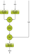
• Dense layer with attention  : We add to a simple dense layer, a pseudo attention mechanism, as in Figure below
• Dense layer 64  :A simple dense layer net with a size of 64 and dropout of 0.5  

The results are summarize on this table : 

There is no significant improvement on model performance in this session. Some models, relying on slightly different electrical parameters (Correlation 100) achieve similar performances, with a gain on MAE and a loss on R2.  

Other methods including different factors fail to deliver performing models, and result in uncorrelated models with a low R2, which seems less exploitable than our previous model.  

We did not use any deep learning architectures, as our actual models (simple architectures) struggle with overfitting.  

This project is part of a project that has received funding from the European Union’s Horizon 2020 research and innovation program under  I-NERGY  grant agreement No 101016508.